Towards cardinal uncertainty quantification in AI
Posted on October 13, 2025 by Michele Caprio[ go back to blog ]
Conformal prediction is an uncertainty representation technique. Given (i) a dataset with \(n\) elements sampled from a homogeneous enough population, (ii) a precision level \(\alpha\) between \(0\) and \(1\), and (iii) a function measuring how every element of the dataset “conforms/is similar to” the other ones, it delivers a conformal prediction region for the \((n+1)\)-th observation. The latter is contained in the conformal prediction region with probability at least \(1-\alpha\). Recently, conformal prediction has seen a surge in popularity given by its widespread adoption in Engineering and AI, two fields that are pervasive to modern-day STEM research.
Introduction
Conformal prediction’s status as an uncertainty quantification tool, though, has remained conceptually opaque: While conformal prediction regions give an ordinal representation of uncertainty (larger regions typically indicate higher uncertainty), they lack the capability to cardinally quantify it (twice as large regions do not imply twice the uncertainty). We adopt a category-theoretic approach to show that—under minimal assumptions—conformal prediction’s cardinal uncertainty quantification capabilities are a structural feature of the method. As a byproduct, we demonstrate that conformal prediction bridges (and perhaps subsumes) the Bayesian, frequentist, and imprecise probabilistic approaches to predictive statistical reasoning.
Uncertainty quantification is a feature of paramount importance to scientific inquiry. To borrow Feynman’s famous words from his report on the space shuttle Challenger accident,
“When using a mathematical model, careful attention must be given to uncertainties in the model.”
Conformal prediction ([1, 2]) is a relatively recent statistical technique that, given some collected evidence coming from a homogeneous enough population, allows one to derive a prediction region that contains the next observation with high probability. Its popularity is due to its relative simplicity, powerful guarantees, and the possibility to wrap it around any statistical, machine learning, and AI method.
Let us illustrate conformal prediction through a simple example. Suppose we record \(n\) height measurements \(y_1,\ldots,y_n \in Y\) from a homogeneous pool of children (age, world region, sex, nutrition, health condition, etc.) such that the sequence of random quantities \(\mathcal{Y}_1,\ldots,\mathcal{Y}_n\) is exchangeable. That is, any permutation of the heights has the same joint distribution. In practical terms, the order in which the kids are measured carries no additional information, so shuffling the data does not affect the analysis; exchangeability is often met in many machine learning and AI applications. Our goal is to predict the next observation \(y_{n+1}\) using a method that is valid or reliable in a certain sense. Usually, prediction methods return a crisp value for \(y_{n+1}\); instead, the goal of conformal prediction is to derive a region that contains \(y_{n+1}\)—the realization of the next element \(\mathcal{Y}_{n+1}\) in the exchangeable sequence—with high probability.
Let \(\mathcal{Y}^{n+1}=(\mathcal{Y}^n,\mathcal{Y}_{n+1}) \) be an \((n+1)\)-dimensional vector consisting of the observable \(\mathcal{Y}^n=(\mathcal{Y}_1,\dots,\mathcal{Y}_n)\) and the yet-to-be-observed value \(\mathcal{Y}_{n+1}\). Consider the transformation \(\mathcal{Y}^{n+1} \rightarrow T^{n+1}=(T_1,\ldots,T_{n+1})\) defined by the rule
\[ T_i := \psi_i \!\left(y^{n+1} \right) \equiv \psi \!\left(y^{n+1}_{-i},y_i \right) \quad\text{for all } i\in\{1, \ldots, n+1\}, \]where \(y^{n+1}:= (y_1,\ldots,y_n,y_{n+1})\), \(y^{n+1}_{-i}:=y^{n+1}\setminus\{y_i\}\), and \(\psi:Y^n \times Y \rightarrow \mathbb{R}\) is a fixed function that is invariant to permutations in its first vector argument. The function \(\psi\), called a non-conformity measure, is constructed in such a way that large values \(\psi_i(y^{n+1})\) suggest that the observation \(y_i\) is “strange” and does not conform to the rest of the data \(y^{n+1}_{-i}\).
The key idea is to define \(\psi_i(y^{n+1})\) in a way that allows us to compare \(y_i\) to a suitable summary of \(y^{n+1}_{-i}\), e.g. \(\psi_i(y^{n+1})=|\mathrm{mean}(y^{n+1}_{-i})-y_i|\), for all \(i\in\{1,\ldots,n+1\}\). Continuing our example, we compare the height of the \(i^\text{th}\) kid to the average height of the others. Notice that the transformation \(\mathcal{Y}^{n+1} \rightarrow T^{n+1}\) preserves exchangeability.
As the value \(\mathcal{Y}_{n+1}\) has not yet been observed, and is actually the prediction target, the above calculations cannot be carried out exactly. Nevertheless, the exchangeability-preserving properties of the transformations described above provide a procedure to rank candidate values \(\tilde{y}\) of \(\mathcal{Y}_{n+1}\) based on the observed \(\mathcal{Y}^n=y^n\).
To operationalize this, we specify a grid of candidate values \(\tilde y\) for the realization of \(\mathcal{Y}_{n+1}\), and, for each such \(\tilde y\), we put \(y_{n+1}=\tilde y\), so that \(y^{n+1}=y^n \cup \{\tilde y\}\). Then, we put \(T_i=\psi_i(y^{n+1})\), for all \(i\in\{1,\ldots,n+1\}\), and finally we evaluate and return
\[ \pi(\tilde{y},y^n):= \frac{1}{n+1}\sum_{i=1}^{n+1} \mathbb{1}\!\left[T_i \geq T_{n+1}\right], \]for each \(\tilde{y}\) on the grid, where \(\mathbb{1}[\cdot]\) denotes the indicator function. The output of this procedure is the conformal transducer, a data-dependent function \(\tilde{y} \mapsto \pi(\tilde{y},y^n) \in [0,1]\) that can be interpreted as a measure of plausibility of the assertion that \(\mathcal{Y}_{n+1} = \tilde{y}\), given data \(y^n\).
The conformal transducer \(\pi\) plays a key role in the construction of conformal prediction regions. For any \(\alpha\in [0,1]\), the \(\alpha\)-level conformal prediction region is defined as (see Chapter 4.5 of [1])
\[ \mathscr{R}_\alpha^\psi(y^n):=\{y_{n+1}\in Y : \pi(y_{n+1},y^n)> \alpha\}, \]and it satisfies \(P\!\left[\mathcal{Y}_{n+1}\in\mathscr{R}_\alpha^\psi(y^n)\right] \geq 1-\alpha\), uniformly in \(n\) and in \(P\) [1]. That is, the guarantee is satisfied for all \(n\in\mathbb{N}\) and all exchangeable distributions \(P\), and it holds regardless of the choice of the non-conformity measure \(\psi\). However, the choice of \(\psi\) is crucial in terms of the efficiency of conformal prediction, that is, the size of the prediction regions.
Results
Despite its merits, conformal prediction suffers from a critical shortcoming. Indeed, a conformal prediction region only gives an ordinal representation of uncertainty: The diameter \(\mathrm{diam}(\mathscr R)\) of a conformal prediction region \(\mathscr R\subseteq Y\) is only defined up to strictly order-preserving (monotone) transformations. Therefore,
\[ \mathrm{diam}\bigl(\mathscr{R}_1\bigr)= 2\,\mathrm{diam}\bigl(\mathscr{R}_2\bigr) \]does not imply that \(\mathscr{R}_1\) is twice more uncertain than \(\mathscr{R}_2\). In general, conformal prediction’s intrinsic cardinal uncertainty quantification capabilities have been a traditionally difficult problem to study. This is also true for many AI and machine learning uncertainty quantification methods [3]. To solve it, we use a category-theoretic approach [4].
Cardinal uncertainty quantification Capabilities of Conformal Prediction
We first cast conformal prediction as a set-valued function (also called a correspondence), \(\kappa: [0,1] \times Y^n \times \mathscr{F} \rightrightarrows Y\), \((\alpha,y^n,\psi) \mapsto \kappa(\alpha,y^n,\psi)\), where \(\mathscr{F}\) is a collection of non-conformity measures, and
\[ \kappa(\alpha,y^n,\psi) := \Bigg\{y_{n+1}\!:\! \underbrace{\frac{1}{n+1}\sum_{i=1}^{n+1} \mathbb{1}\!\left[\psi \!\left(y^{n+1}_{-i},y_i \right) \geq \psi \!\left(y^{n+1}_{-(n+1)},y_{n+1} \right)\right]}_{=: \pi(y_{n+1},y^n)} > \alpha\Bigg\}. \]It is easy to see, then, that \(\kappa(\alpha,y^n,\psi) \equiv \mathscr{R}_\alpha^\psi(y^n)\).
Category theory studies mathematical structures (called categories) of objects and their relations (called morphisms) [5]. It also inspects connections (called functors) between different such structures. Two of the main advantages of working in this field are (i) to be able to transport problems from one area of mathematics to another area, where solutions are sometimes easier, and then transport back to the original area; and (ii) to provide the means to distinguish between general (“categorical”) problems and specific problems [6].
We introduce a new category, \(\mathbf{UHCont}\), whose objects are topological spaces, and whose morphisms are upper hemicontinuous correspondences. Fix any \(n \in \mathbb{N}\), and consider the following conditions:
- \(Y\) is compact Hausdorff, endowed with the Borel \(\sigma\)-field \(\mathcal{B}(Y)\).
- Each \(\psi\in\mathscr{F}\) is jointly continuous on \(Y^{n}\times Y\), and \(\mathscr{F}\) is endowed with the uniform (\(\sup\)-norm) topology.
- The credibility level \(\alpha\) satisfies \(\alpha\notin S_{n+1}:= \bigl\{0, \tfrac{1}{n+1}, \tfrac{2}{n+1}, \ldots, \tfrac{n}{n+1}, 1\bigr\}\).
- The space of (finitely additive) probabilities \(\mathrm{Prob}\) on \(Y\) is endowed with the weak\(^\star\) topology, and the space \(\mathscr C\subset 2^{\mathrm{Prob}}\) of convex and weak\(^\star\)-closed subsets of \(\mathrm{Prob}\) (called credal sets [7]) is endowed with the Vietoris topology.
In our running kids’ heights example, to satisfy them, it is enough e.g. to let \(Y=[0,200]\) (where the units are centimeters), to pick \(\psi_i(y^{n+1})=|\mathrm{mean}(y^{n+1}_{-i})-y_i|\) for all \(i\), as we wrote before, and to select an \(\alpha\) outside of \(S_{n+1}\) to satisfy these conditions. Under these assumptions, conformal prediction’s intrinsic cardinal uncertainty quantification capabilities are shown.
Intuitively, conformal prediction is equivalent to first deriving a set of probabilities \(\mathcal{M}\in\mathscr C\) from the available data \(y^n\), and then using \(\mathcal{M}\) to obtain a prediction region that is equivalent to the conformal prediction region \(\mathscr{R}_\alpha^\psi\) [8]. This is expressed formally below.
The set \(\mathcal{M}\) is used to cardinally quantify different types of uncertainties (epistemic and aleatoric, that is, reducible and irreducible) [9, 10, 11]. For example, Abellán et al. [9] posit that the epistemic uncertainty is captured by the generalized Hartley measure \(\mathrm{GH}(\mathcal{M})\) of \(\mathcal{M}\), which measures the (logarithm of the) largest number \(n(\mathcal{M})\) of pairwise fully contradictory probability measures in \(\mathcal{M}\). If \(\mathrm{GH}(\mathcal{M}_1) = 2\,\mathrm{GH}(\mathcal{M}_2)\), then \(\mathcal{M}_1\) encodes twice as much EU as \(\mathcal{M}_2\), which formally means that \(n(\mathcal{M}_1)=n(\mathcal{M}_2)^2\).
Theorem. Assume the conditions above hold, and that \(\sup_{\tilde y \in Y} \pi(\tilde y,y^n)=1\). Consider any \(\alpha \in [0,1]\) that satisfies (iii). Then the Full Conformal Prediction Diagram commutes in \(\mathbf{UHCont}\); in particular, \(\mathrm{IHDR}_\alpha \circ \mathrm{CRED} = \kappa_\alpha\). Here, \(\mathrm{CRED}\) extracts the credal set \(\mathcal{M} \in \mathscr{C}\) from the data, and \(\mathrm{IHDR}_\alpha\) derives an (imprecise) \(\alpha\)-level confidence region from \(\mathcal{M}\), called the imprecise highest density region [12].
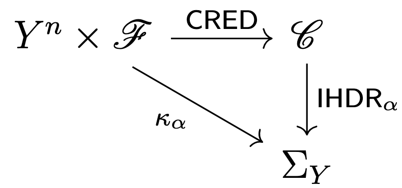
Part of the Full Conformal Prediction Diagram
Sketch of proof. (a) Under the stated assumptions, \(\mathrm{CRED}\), \(\kappa_\alpha\), and \(\mathrm{IHDR}_\alpha\), \(\alpha \in [0,1]\setminus S_{n+1}\), are morphisms of \(\mathbf{UHCont}\); (b) the assumptions are minimal: removing any of them invalidates the statement. The result then follows from the equality of the \(\alpha\)-level IHDR of \(\mathcal{M}\) and the \(\alpha\)-level conformal prediction region [8, Proposition 5].
A similar result, under essentially the same conditions, holds if we consider the Full Conformal Prediction Diagram embedded in the category \(\mathbf{WMeas}_{\mathrm{uc}}\), whose objects are measurable Polish spaces, and whose morphisms are weakly measurable, uniformly compact-valued correspondences.
These results tell us that the Full Conformal Prediction Diagram commutes when we focus either on the continuity or on the measurability aspects (fundamental, but generally non-equivalent, concepts in functional analysis) of the conformal prediction correspondence \(\kappa\). This further testifies that, under our assumptions, (cardinal) uncertainty quantification is a built-in feature of Conformal Prediction methods. See the figure below for a visual representation of our findings.
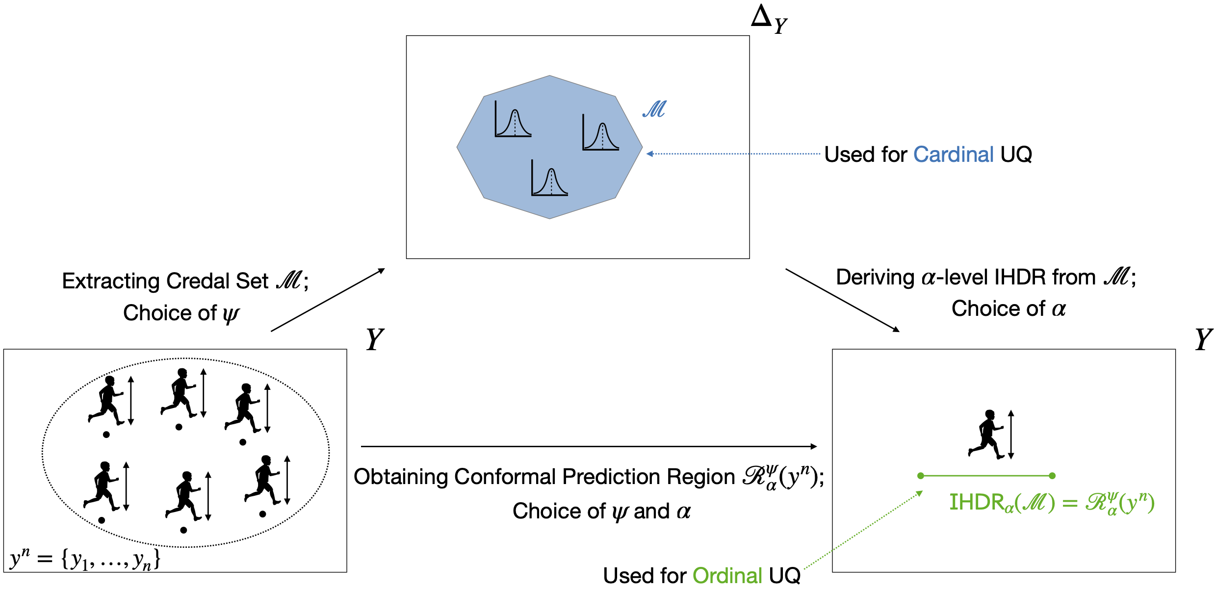
A visual representation of our findings. Kids’ heights \(y_1,\ldots,y^n\) are represented by points below their figurines. From the training set \(y^n\), we can extract credal set \(\mathcal{M}\), used for cardinal uncertainty quantification, and then derive an IHDR (green segment) for the \((n+1)^\text{th}\) kid. This IHDR is equivalent to the conformal prediction region that can be directly extracted from \(y^n\), used for ordinal uncertainty quantification.
Bridging Bayesian, frequentist, and imprecise reasoning
Another interesting result pertains to how conformal prediction bridges Bayesian, frequentist, and imprecise probabilistic predictive reasoning. To see this, let \(\Theta\) be a parameter space, and let \(\Delta^\mathrm{dens}_\Theta\) be the space of probabilities on \(\Theta\) that admit densities with respect to some dominating measure \(\lambda_\Theta\). Suppose the usual minimal technical machinery needed to ensure that the posterior predictive \(p_P(y_{n+1} \mid y^n)\) is (a) well-defined, and (b) varies continuously in both the data \(y^n\) and the prior \(P \in \Delta^\mathrm{dens}_\Theta\), holds [4, Conditions (v)–(x)]. If we pick as non-conformity measure the negative posterior predictive density, i.e. \(\psi (y^{n+1})= -p_P(y_{n+1} \mid y^n)\), then the conformal prediction region coincides asymptotically with the \(\alpha\)-level set of the posterior predictive distribution.
Theorem. Assume the conditions above and [4, (v)–(x)] hold, and that \(\sup_{\tilde y \in Y} \pi(\tilde y,y^n)=1\). Then the corresponding diagram (linking \(\mathrm{CRED}\), \(\mathrm{IHDR}_\alpha\), the Bayesian conformal construction, and the \(\alpha\)-level posterior predictive quantile set) commutes asymptotically in probability in \(\mathbf{UHCont}\).
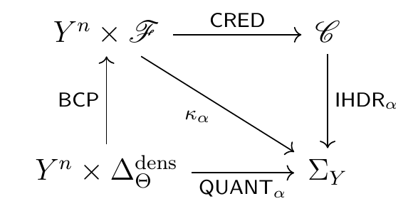
Full Conformal Prediction Diagram
Sketch of proof. (a) Under the stated assumptions, all correspondences are morphisms of \(\mathbf{UHCont}\); (b) the conditions are minimal. Then, the \(\alpha\)-level set of the posterior predictive density approaches asymptotically in probability (in the Hausdorff distance) the \(\alpha\)-level conformal prediction region. Finally, the result follows from [8, Proposition 5].
This confirms the intuition in [13] that conformal prediction is a bridge between the Bayesian, frequentist, and imprecise approaches to predictive statistical reasoning. Indeed, the model-based Bayesian and imprecise (via the credal set \(\mathcal{M}\)) methods, and the model-free conformal construction, yield (asymptotically) the same \(\alpha\)-level prediction region, showing deep connections between these three only apparently far-apart mechanisms.
Discussion
This work opens up the study of categorical conformal prediction and hints at many unsolved problems. For example, it is an open question how to leverage the structure of the functional-analysis-flavored categories \(\mathbf{UHCont}\) and \(\mathbf{WMeas}_\mathrm{uc}\) to learn further aspects of the conformal prediction methodology. In particular, because the morphisms of these categories are set-valued functions, it is interesting to study whether the Kleisli categories [5, Section 5.1] arising from subcategories of \(\mathbf{UHCont}\) and \(\mathbf{WMeas}_\mathrm{uc}\) admitting a monad allow us to establish new properties of conformal prediction. It is also left to inspect whether studying conformal prediction as a morphism of different categories can allow us to remove the need for assumptions altogether, particularly compactness of the state space \(Y\).
Acknowledgements
We thank Sam Staton, Paolo Perrone, Nicola Gambino, Yusuf Sale, Eyke Hüllermeier, Sangwoo Park, Alessandro Zito, Nina Gottschling, and Siu Lun Chau for comments and references.
References
[1] Vladimir Vovk, Alexander Gammerman & Glenn Shafer. Algorithmic Learning in a Random World. Springer, 2025.
[2] Anastasios N. Angelopoulos, Rina Foygel Barber & Stephen Bates. Theoretical Foundations of Conformal Prediction. Cambridge University Press, 2025. arXiv:2411.11824 [math.ST]
[3] Yaniv Ovadia, Emily Fertig, Jie Ren, Zachary Nado, D Sculley, Sebastian Nowozin, Joshua V. Dillon, Balaji Lakshminarayanan & Jasper Snoek. Can you trust your model’s uncertainty? Evaluating predictive uncertainty under dataset shift. In: Proceedings of the 33rd International Conference on Neural Information Processing Systems (NeurIPS 20219). Curran Associates Inc., 2019. arXiv:1906.02530
[4] Michele Caprio. The joys of categorical conformal prediction. 2025. arXiv:2507.04441 [stat.ML]
[5] Paolo Perrone. Starting Category Theory. World Scientific, 2024.
[6] Bodo Pareigis. Lecture Notes in Category Theory. Department of Mathematics of LMU Munich, 2004.
[7] Isaac Levi. The Enterprise of Knowledge. MIT Press, 1980.
[8] Michele Caprio, Yusuf Sale & Eyke Hüllermeier. Conformal prediction regions are imprecise highest density regions. In: Proceedings of the Fourteenth International Symposium on Imprecise Probabilities: Theories and Applications (ISIPTA 2025), PMLR vol. 290, p. 47–59, 2025. arXiv:2502.06331 [stat.ML]
[9] Joaquín Abellán, George Jiří Klir & Serafín Moral. Disaggregated total uncertainty measure for credal sets. In: International Journal of General Systems 35:1, p. 29–44, 2006.
[10] Eyke Hüllermeier & Willem Waegeman. Aleatoric and epistemic uncertainty in machine learning: an introduction to concepts and methods. In: Machine Learning 110:3, p. 457–506, 2021.
[11] Siu Lun Chau, Michele Caprio & Krikamol Muandet. Integral Imprecise probability metrics. 2025. arXiv:2505.16156 [stat.ML]
[12] Frank P.A. Coolen. Imprecise highest density regions related to intervals of measures. In: Memorandum COSOR:9254, Technische Universiteit Eindhoven, 1992.
[13] Ryan Martin. Valid and efficient imprecise-probabilistic inference with partial priors, II. General framework. 2022. arXiv:2211.14567 [stat.ME]
About the author

Michele Caprio is a Lecturer (Assistant Professor) in Machine Learning and Artificial Intelligence at The University of Manchester, and a member of the Manchester Centre for AI Fudamentals. His general interest is probabilistic machine learning, and in particular the use of imprecise probabilistic techniques to investigate the theory and methodology of uncertainty quantification in machine learning and artificial intelligence. Recently, he won the IJAR Young Researcher and the IMS New Researcher Awards, he was elected Fellow of the Cambridge Philosophical Society, and nominated Action Editor of Transactions on Machine Learning Research and Associate Editor of ACM Transactions on Probabilistic Machine Learning.